OpenHyPE: OpenHygrisC Data Processing for Education
- Project funded by the Federal State of Northrhine-Westphalia (NRW)
- Project duration: 15.12.2021 - 30.06.2023

0. Abstract
The State Agency for Nature, Environment and Consumer Protection (LANUV) of the federal state of North Rhine-Westphalia (NRW) provides extensive quantitative and qualitative groundwater monitoring data. This contributes to the fulfillment of the European Water Framework Directive as well as the EU INSPIRE Directive for an open interoperable spatial data infrastructure.
NRW operates its own water-related data portal ELWAS-WEB, which also provides the groundwater database HygrisC. ELWAS and HygrisC are not easy to use and provide only limited exploratory data analysis capabilities to the public.
However, the state publishes much of its groundwater data as an open data archive called OpenHygrisC, which contains several data tables in csv format. In particular, the big data in the measurement table, which contains all time series with more than 3.6 million individual measurements (table rows), and the table with the spatial coordinates of the groundwater monitoring wells require the use of a spatially enabled object-relational database management system (Spatial ODBRMS) and extensive data engineering before insertion into the database.
The goal of the OpenHyPE project is to develop a first set of Open Educational Resources (OER) to train the setup, filling and use of a geospatial-temporal database with the OpenHygrisC data. Due to the graduated level of difficulty, the project addresses students from secondary schools as well as universities in the state of North Rhine-Westphalia and beyond.
All software products used are Free and Open Source Software (FOSS). The database, which we call OpenHyPE DB, is based on PostgreSQL / PostGIS and establishes the center of the system for environmental data analysis and presentation. The OER demonstates how the geographic information system QGIS as well as Python programs in the JupyterLab development environment interoperate with the OpenHyPE DB to select, analyze and display the data in the form of time dependent maps or time series. We use Python and Jupyter from the Anaconda distribution.
The start-up funding for the OpenHyPE project is used to raise awareness of the NRW's valuable open environmental data collection among young people as well as to contribute to interdisciplinary STEM promotion in general and education for sustainable development (ESD) in particular by linking environmental science and computer science.
1. Introduction
1.1 Problem Description
The state of North Rhine-Westphalia (NRW) operates comprehensive and professional measurement networks for the collection of environmental data through the LANUV. As part of Open.NRW and driven by the INSPIRE Directive of the European Union as well as other directives such as the EU Water Framework Directive (WFD), the state of NRW makes extensive data products openly accessible and freely usable on various platforms (Free and Open Data).
The state of NRW is a pioneer in Germany in providing open and (cost)free geodata. These data are a real treasure and form the basis for potentially massive knowledge gains in the field of environmental and nature conservation. Nevertheless, it seems that only a comparatively small group of people really uses this potential. Therefore, the OpenHyPE project has set itself the task of integrating this data stock into university teaching and developing corresponding freely accessible teaching material that can be used not only by students but also, to some extent, by pupils to learn the basics of environmental data processing. The start-up funding will be used to implement the first steps of developing such training material.
We follow the paradigm of “problem based learning”: the necessary knowledge and skills are identified and taught based on a concrete socially relevant problem. The solution of the problem identified as significant is the motivation for learning.
At the beginning we want to develop the material on the basis of the problem area “groundwater protection”. The Ministry for Environment, Agriculture, Nature and Consumer Protection NRW (MULNV) operates its own water-related data portal called ELWAS-WEB via the “Landesbetrieb Information und Technik Nordrhein-Westfalen” (IT.NRW). Data from the statewide groundwater database HygrisC are also held in this portal. ELWAS and HygrisC offer limited exploratory data analysis capabilities to outsiders. From the point of view of usability engineering, which deals with the user-friendliness of technical systems, improvements are desirable with regard to usability as well as data analysis possibilities, because exploratory data analysis and data mining in particular help to identify structures and relationships between data. ELWAS and HygrisC are therefore only suitable to a limited extent for teaching the basics of environmental data analysis, but they can be used in the classroom as supporting material.
On the portal OpenGeodata.NRW extensive data with spatial reference - also called geodata - are made available, which often have a time reference, such as land use changes or measurement data series on water quality. Excerpts of the HygrisC groundwater database of the state of NRW, published under the name OpenHygrisC, are also located there. These groundwater data can ideally serve as a basis for building one's own environmental database, which the learners can use to learn about concepts of data management and data analysis.
1.2 Project Goals
The following components are to be realized:
- Development of OpenHyPE geodatabase based on PostgreSQL/PostGIS
to manage spatial and temporal data on groundwater quality and quantity. - Problem-related free online course material (OER), tutorials, video tutorials, instructions, program code,
using Free and Open Source Software (FOSS):- Introduction to the State Agency for Nature, Environmental and Consumer Protection (LANUV).
- Introduction to groundwater protection
- Introduction to the Geographic Information System QGIS
- Introduction to the relational database PostgreSQL and the query language SQL
- Introduction to the geodatabase extension PostGIS
- Introduction to the processing of geodata with the programming language Python
- Installation of the OpenHyPE database management system
- Discussion of the data model and upload of the OpenHygrisC data of the LANUV
- Automatic creation of diagrams on time series of water quality
- Automatic generation of groundwater chemistry maps
- Creating simple dashboards with interactive online graphs and maps
- Introduction to data mining (descriptive statistics, searching for correlations)
2. Implementation
2.1 Data Flow
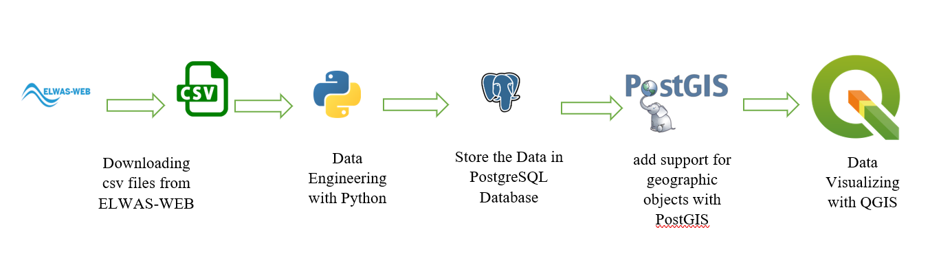 |
| Image 1- Data flow |
2.2 PostgreSQL/PostGIS
PostgreSQL is an open-source object-relational database management system (DBMS) known for its robustness, scalability, and extensive features. It is often referred to as “Postgres” and is one of the most popular and widely used databases in the world. PostgreSQL supports a wide range of data types, including numeric, text, Boolean, date/time, JSON, XML, and more. It provides support for complex queries, indexing, and advanced features such as full-text search, spatial data storage and querying, and transactional processing with ACID (Atomicity, Consistency, Isolation, Durability) properties.
PostgreSQL follows the SQL (Structured Query Language) standard, and it also provides additional features beyond the standard SQL specification. It supports stored procedures, triggers, and views, allowing developers to define custom business logic within the database itself.
PgAdmin is an open-source administration and development platform for PostgreSQL. It is a graphical user interface (GUI) tool that provides a convenient way to manage and interact with PostgreSQL databases.
PostGIS: PostGIS is an open-source spatial database extension for PostgreSQL. It adds support for geographic objects and spatial functions to the PostgreSQL database, enabling the storage, retrieval, and analysis of geospatial data. Geographic data such as points, lines, polygons, and multi-dimensional geometries can be stored and manipulated within your PostgreSQL database using PostGIS. The capabilities of the database are extended by PostGIS to handle spatial data types, indexing, and spatial operations. PostGIS has gained popularity in a variety of applications, including mapping, geolocation-based services, environmental analysis, urban planning, and transportation. Its combination with the power and versatility of PostgreSQL makes it a robust solution for managing and analyzing geospatial data in a relational database environment.
The below image shows the PGadmin tool.
 |
| image 2- PGadmin |
Watching the below videos to understand how we can create schemas and tables in the PostgreSQL database.
| video1- Create Schema in PGadmin | video2- Create tables in PGadmin |
Create a database and schema based on the above video.
2.3 Data Engineering
2.3.1 Downloading the Data
In the first step, The data must be downloaded from here. To complete the process, download and extract the initial zip file, which contains four CSV files and one set of instructions. Refer to image 3 for guidance on selecting the appropriate zip file.
 |
| image 3- Download the data |
After the above zip file has been extracted, the four CSV files and the instruction file can be considered, with a strong recommendation to read the instruction file first.
2.3.2 Python
Python is a high-level, interpreted, and general-purpose programming language known for its simplicity and readability. It was created by Guido van Rossum and first released in 1991. Python emphasizes code readability and has a design philosophy that emphasizes clear, concise syntax, making it easier to write and understand code. Python is used in several ways such as:
- AI and machine learning
- Data analytics
- Data visualisation
- Programming applications
In this project, we have used Python for data engineering, data pre-processing, and data analysis. Jupyter Notebook is used in this project to write Python codes. The Jupyter Notebook is an open-source web application that data scientists can simply write the code for and make it easier to document. Simply, we can combine Python codes, text, images, comments, and the result of the codes on the same page. The below image shows how code, text, and the result of the code can be seen on a single page.
 |
| image 4- combination of code and text in the jupyter notebook |
2.3.3 Anaconda
Anaconda is an open-source distribution for python and R. It is used for data science, machine learning, deep learning, etc. With the availability of more than 300 libraries for data science, it becomes fairly optimal for any programmer to work on anaconda for data science Anaconda is used in this project. An environment on Anaconda has been created to install all the packages needed for this project.
| Video 3- How to install Anaconda on Windows |
| Video 4- How to install Anaconda on Mac OS X |
Environment in Anaconda: A conda environment is a directory that contains a specific collection of conda packages that are used in the project.
How to create Conda environment: The below video shows how to create a Conda environment, how to activate it, how to install different packages on the environment and how to deactivate the environment.
| Video 5- How to create Conda environment |
Python packages: Python packages are collections of modules that provide additional functionality and tools to extend the capabilities of the Python programming language. Packages are typically distributed and installed using package managers such as pip (the default package manager for Python) or conda.
To get more details about conda environment, I highly recommend visiting the below webpage.
https://towardsdatascience.com/manage-your-python-virtual-environment-with-conda-a0d2934d5195
openhype environment: For this project, an “openhype” environment was created to install all the required packages. This environment ensures that all the necessary dependencies are properly installed and configured.
Several packages are related to data science but in this project, we have used the below packages. There are two ways to install the below packages:
install a package manually: In this way you need to install each package manually into openhype environment by the command prompt.
- pandas: Pandas is a popular open-source Python library for data manipulation and analysis. It provides easy-to-use data structures, such as DataFrame, Series, and Index, that are designed to handle structured data efficiently.
In this project, pandas was utilized to read the CSV files, clean the data, and perform data engineering tasks. To install Pandas, execute the following Python code within the openhype environment in the Anaconda prompt:
conda install pandas
- sqlalchemy: SQLAlchemy is a popular open-source SQL toolkit and Object-Relational Mapping (ORM) library for Python. It provides a set of high-level APIs that allow developers to interact with relational databases using Python code.
conda install sqlalchemy
- psycopg2: Psycopg2 is a PostgreSQL adapter for Python. It provides a Python interface for interacting with PostgreSQL databases, allowing developers to connect to a PostgreSQL database server, execute SQL queries, and perform database operations using Python code.
conda install psycopg2
- geopandas: Geopandas is an open-source Python library built on top of Pandas and other geospatial libraries. It extends the capabilities of Pandas by adding support for geospatial data, enabling users to work with spatial data in a tabular format.
conda install --channel conda-forge geopandas
Certain packages require the specification of a channel for installation. This is why the above code includes the channel specification to ensure the correct installation.
- jupyter notebook: Jupyter Notebook is an open-source web-based interactive computing environment that allows users to create and share documents containing live code, visualizations, explanatory text, and more. It supports various programming languages, including Python, R, and Julia.
conda install jupyter notebook
To ensure the successful installation of all the aforementioned packages, it is crucial to install them within the openhype environment using the Anaconda prompt.
Load all the packages into the environment by a YAML file: To streamline the installation process for all the required packages in this project, it is recommended to create an environment named “Openhype” and load a YAML file containing the package specifications. The contents of the “openhype.yml” file, as shown in the image below, encompass all the necessary packages.
 |
| image 5- openhype.yml |
The following code allows you to create an environment based on the yml file. Keep in mind that the YAML file should be in the same directory as your Anaconda installation. If the file is located elsewhere, you will need to provide the full path to the file in the code. openhype.yml can be found from here
conda env create -f openhype.yml
How to create a yml file for the environment: With the below code you can export the yml file from the existing environment.
conda env export > openhype.yml
Since the four CSV files have been downloaded in the previous chapter, it is time to read the CSV files and initiate the cleaning process to make them ready for importation into our database.
Refer to the code section in our Notebook for more information Github (the below image).
 |
| image 6- Github |
There below four notebooks should be run separately, in order to import data into the database.
- import_gemeinde.ipynb:
In this notebook, we will import the data of all geminde into the database.
- import_katalog_stoff.ipynb:
In this notebook, we will import the data of all the catalogue substances into the database.
- import_messstelle.ipynb:
In this notebook, we will import the data of all stations into the database.
- import_messwert.ipynb:
In this notebook, we will import the data of all values into the database.
2.4 Observation Data in the Database
After successfully downloading, cleaning, and importing the data into the database in the previous section, it is now time to examine the data within the database. Since we are working with a PostgreSQL database, we can utilize SQL commands to retrieve and analyze the data. Let's run some basic SQL commands to gain insights into the data.
To view our tables, we can use the following code. It selects all the columns from the “hygrisc” schema, which contains our tables. We limit the output to the first 100 rows to avoid overwhelming results.
select * from hygrisc.messwert limit 100;
Image 7 illustrates the outcome of the aforementioned command executed in PGAdmin. It displays the resulting data obtained from the execution of the provided SQL command.
 |
| image 7- messwert table in databse |
Now with the above SQL command, we are able to see the other three tables that we have (The below codes).
select * from hygrisc.messstelle limit 100;
select * from hygrisc.katalog_stoff limit 100;
select * from hygrisc.katalog_ge limit 100;
Now we want to see more details for our tables and we will run the below codes.
Count the rows of each table: With the below code, we can see how many rows we have in each table.
select count (*) from hygrisc.messwert;
select count (*) from hygrisc.messstelle;
Filter the data based on Nitrate only: To determine the substance number of Nitrate, we need to retrieve the corresponding information from the database.
select * from hygrisc.katalog_stoff where name like 'Ni%';
 |
| Image 8- Find out the substance number (stoff_nr) of Nitrate |
According to the information presented in “Image 8,” the substance number (stoff_nr) of Nitrate is 1244
select * from hygrisc.messwert where stoff_nr = '1244';
Now we can filter the messwert table based on Nitrate. In this step, We can save this new table as a new “view”.
What is a view: a view is a virtual table that is derived from one or more existing tables or other views. A view does not store data physically but rather provides a way to present data from underlying tables in a structured and organized manner. It acts as a predefined query that can be used to retrieve and manipulate data. The below code creates views:
create view hygrisc.nitrat as (select * from hygrisc.messwert where stoff_nr = '1244');
We now have a “nitrat” view, which can be accessed just like a table using the following code. This view is filter of our messwert table based on “1244” which is “Nitrate”
select * from hygrisc.nitrat ;
Group by the two tables: the Group by clause is used to group rows based on one or more columns in a table. When working with two tables, you can perform a GROUP BY operation to group the data based on common values from both tables. In this section, we want to group by our two tables (messwert and messstelle) only in Nitrate. These two tables have a column messstelle_id which means station id.
select messstelle_id, count(*) from hygrisc.messwert where stoff_nr = '1244' group by messstelle_id;
 |
| Image 9- Group by the two tables (messwert and messstelle) |
Image 9 shows that each station id has how many single measurements for the Nitrate only. I highly recommend opening the below website to get more deep into how “group by” works and how we can use it.
https://www.w3schools.com/sql/sql_orderby.asp
| Video 6- How group by works |
Maximum date in nitrat table:
select * from hygrisc.nitrat where datum_pn = (select max(datum_pn) from hygrisc.nitrat);
 |
| Image 10- Maximum of the date in the nitrat table |
As we can see in Image 10, the maximum date is 2021-08-17
Minimum date in nitrat table:
select * from hygrisc.nitrat where datum_pn = (select min(datum_pn) from hygrisc.nitrat);
 |
| Image 11- Minimum of the date in the nitrat table |
As we can see in Image 11, the minimum date is 1951-04-30
Create geometry column in messstelle table: In this section, we want to create a geometry column from e32 and n32 columns from the messstelle table. With the below code, we are able to create a new column and we set the name as geom
ALTER TABLE hygrisc.messstelle ADD COLUMN geom geometry(Point, 25832);
UPDATE hygrisc.messstelle SET geom = ST_SetSRID(ST_MakePoint(e32, n32), 25832);
 |
| Image 12- Geom column |
The “messstelle” table has been enhanced with an additional column called “geom,” which contains the geometry information representing the location of each station.
Merge two tables:
In this section, we aim to merge the “messwert” and “messstelle” tables based on the common column, “messstelle_id.” To achieve this, we will select the desired columns from each table and then perform the merge based on the “messstelle_id” column.
select t1."messstelle_id", t1."name", t1.geom, t2."stoff_nr", t2."messergebnis_c", t2."masseinheit",
t2."datum_pn", t2."messergebnis_cm" from  hygrisc.messstelle t1 , hygrisc.nitrat t2
where t1."messstelle_id" = t2."messstelle_id";
 |
| Image 13- Merge tables |
In order to have the above SQL command available as a new view for the subsequent section in QGIS, we should store it accordingly.
create view hygrisc.nitrat_geom as (select t1."messstelle_id", t1."name", t1.geom, t2."stoff_nr", t2."messergebnis_c", t2."masseinheit",
 t2."datum_pn", t2."messergebnis_cm" from  hygrisc.messstelle t1 , hygrisc.nitrat t2
where t1."messstelle_id" = t2."messstelle_id")
2.5 QGIS
QGIS is a free and open-source geographic information system (GIS) software. It provides a wide range of tools and functionalities for visualizing, analyzing, and managing geospatial data. QGIS supports various data formats and allows users to create, edit, and publish maps.
You can download QGIS for free from the below link.
The below video shows how to download and install QGIS for Windows which is highly recommended to watch before installing it.
| Video 7- How to download and install QGIS |
To gain a better understanding of QGIS, I recommend watching the following video, which provides valuable insights and guidance on using the software.
| Video 8- Get to know QGIS |
Create a time series video: In this section, our objective is to generate a time series video depicting the changes in nitrate concentration over time in North Rhine-Westphalia, the most populous state in Germany. To begin, we must download the shapefile for North Rhine-Westphalia and import it into QGIS for further analysis and visualization.
Three below shapefiles need to be downloaded
- entire state shapefile (dvg1bld_nw.shp)
- kreis shapefile (dvg1krs_nw.shp)
- Gemeinde shapefile (dvg1gem_nw.shp)
All three shapefiles can be downloaded from here. After downloading the shapefiles, we can proceed to load them into QGIS for visualization and analysis. The below video shows how to load the shapefile in QGIS.
| Video 9- How to import shapefile in QGIS |
Now we can see the map of NRW, kreis and Gemeinde. There are two options to create a video for time series.
Locally with shapefile: In here, we need to have a shapefile that consists of the nitrate concentration over time. download the notebook from here and run the Python codes to create two shapefiles. then we should load these two shapefiles to the QGIS. The first shapefile consists of all stations in NRW and the second one consists of the nitrate concentration.
The below video shows how we can load shapefiles to QGIS.
| Video 10- How to load shapefile in QGIS |
Connect to Database: The below video shows how we can connect our QGIS to Database and load the file from Database.
| Video 11- How to connect database to QGIS and load the files |
3 Dashboard
In this section, the process of creating an interactive dashboard for our data will be explored. An interactive dashboard is a versatile tool that allows data to be interacted with, analyzed, visualized, and key information to be monitored by users.
This section discusses two approaches to creating a dashboard. The objective of this dashboard is to provide a user-friendly and interactive interface for data exploration and visualization, accessible even to non-programmers. Such a dashboard plays a crucial role in enhancing data comprehension and is widely utilized by managers and decision-makers to facilitate informed decision-making processes.
One notable example of this type of dashboard is the Covid-19 dashboard, which has gained widespread usage worldwide, including in Germany. The Covid-19 dashboard provides users with valuable insights into the number of new cases and deaths reported over various time periods. It helps individuals track the progression of the pandemic and understand the impact it has had on different regions and countries.
In our specific case, the objective is to develop a straightforward dashboard that showcases the map of North Rhine-Westphalia (NRW) alongside the concentration rates of Nitrate and Sulfate at different time intervals. This dashboard will provide a visual representation of the spatial distribution of these pollutants and enable users to observe any temporal variations in their concentrations within NRW.
Plotly Dash:
Plotly: Plotly is a computing company located in Montreal, Canada. They develop online data analytics and visualization tools. Plotly offers online graphing, analytics, and statistics tools for their users, as well as scientific graphing libraries for Python, R, MATLAB, Perl, Julia, Arduino, and REST. Plotly offers several open-source and enterprise products such as Dash which have been used for creating simple and interactive dashboards in this project.
Dash: Dash is a framework to build data apps rapidly not only in Python but also in R, Julia, and F#. According to Plotly's official website, Dash is downloaded 800,000 times per month which shows that nowadays Dash getting more popular. Dash is a great framework for anyone who uses data with a customised user interface. Through a couple of simple patterns, Dash eliminated all of the technologies as well as protocols that are needed to make a full-stack web app with interactive data considerations. Another good feature is that Dash is running on web browsers so it means that no other application needs to run it.
To learn more about creating a dashboard with Plotly Dash, you can follow the link provided below. This resource contains comprehensive tutorials that guide you through the process of building a simple dashboard using Plotly Dash. These tutorials will provide you with step-by-step instructions and examples to help you create interactive and visually appealing dashboards using Plotly Dash.
https://www.youtube.com/c/CharmingData
Dash is also offering some dashboards examples which could be really nice and helpful to get ideas. | Click here for Dash gallery
All the source codes of the dash gallery are available in | here
Dashboard Design: I have developed a web application dashboard that effectively visualizes time series data for Nitrate and Sulfate. The image below shows the main page of our dashboard.
 |
| Image 14- Main page of the dashboard |
In order to run the above dashboard on your local system, you need to do the following:
Click here and pull the repository
direct to the “Dashboard” folder, then all the Python codes and SQL queries are available to run the application.
There is a yml file inside the folder which name is “dashboard_environment”. This yml file will create an environment with all the necessary packages which you will need to run the application. The first step needs to load this file to the Anaconda, if you are not sure how to do that please refer to the 2.3.3 Anaconda section.
The next step is to add the credentials (Username, DB name, password and …) of the database to the “credential_temp” file.
And the last step is to run the “app.py” inside the new environment that you have already created with the help of “dashboard_environment.yml”
4. Result
Nitrate concentration 2000-2010
The video below shows the concentration of nitrate in North Rhine-Westphalia (NRW) from 2000 to 2010. This visualization was created using QGIS 3.16. By watching the video, you can observe the temporal changes in nitrate levels across NRW during the specified time period.
Nitrate concentration 2010-2020
The video below shows the concentration of nitrate in NRW from 2010 to 2020. The video was created with QGIS 3.16
Sulfat concentration 2000-2010
The video below shows the concentration of sulfate in NRW from 2000 to 2010. The video was created with QGIS 3.16
Sulfat concentration 2010-2020
The video below shows the concentration of sulfate in NRW from 2010 to 2020. The video is created with QGIS 3.16
5. Project codes
Weitere Infos
- EOLab-Wiki-Seiten zum Thema Grundwasserdaten in NRW