Table of Contents
Environmental Monitoring Research Project 2021
Intro to Tasmota, IoT, and NIG (NIG: Node-RED, InfluxDB, Grafana)
- More on Tasmota with WEMOS D1 Mini (ESP8266)
Student Pages
1. Problem description
The city of Moers has bought a lot of new trash bins. In order to be able to monitor the filling level of these trash bins, the trash bins have to be equipped with appropriate hardware and software. This project can be seen as a first prototype which goes through the whole process from the collection of the data to the storage and visualization of the data. We use technologies that are also known from the smart city context.
2. Methods and Tools
For our project, we have used LoRaWAN (Low-power wide-area-network), MQTT (MQ Telemetry Transport), TTN (The Things Network), and, Node-RED to efficiently transmit data between devices and the database.
Before we can describe what is LoRaWAN first we need to understand what is LoRa. LoRa is a radio modulation technique that is essentially a way of manipulating radio waves to encode information using a chirped (chirp spread spectrum technology), multi-symbol format. LoRa as a term can also refer to the systems that support this modulation technique or the communication network that IoT applications use.
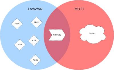
| Figure 1: MQTT & LoRaWan |
The main advantages of LoRa are its long-range capability and its affordability. A typical use case for LoRa is in smart cities, where low-powered and inexpensive internet of things devices (typically sensors or monitors) spread across a large area send small packets of data sporadically to a central administrator.LoRaWAN is a low-power, wide-area networking protocol built on top of the LoRa radio modulation technique. It wirelessly connects devices to the internet and manages communication between end-node devices and network gateways. The usage of LoRaWAN in industrial spaces and smart cities is growing because it is an affordable long-range, bi-directional communication protocol with very low power consumption — devices can run for ten years on a small battery. It uses the unlicensed ISM (Industrial, Scientific, Medical) radio bands for network deployments.
An end device can connect to a network with LoRaWAN in two ways:
Over-the-air Activation (OTAA): A device has to establish a network key and an application session key to connect with the network. Activation by Personalization (ABP): A device is hardcoded with keys needed to communicate with the network, making for a less secure but easier connection. In our project OTAA is used for the activation of the end device. Before OTAA can be used the end device needs to store its DevEUI, AppEUI and Appkey. The AppEUI is required by the network server which is storing the AppEUI of the end device. The AppEUI is used as a unique indentifier for the application server. The AppKey is responsible for the integrity of the message by generating the Message Integrity Code (MIC). AppKey is also stored by the network server. Using MIC a join-request is sent to the network server. The message contains the DevEUI, AppEUI and the DevNonce. DevNonce is a randomly generated number. After that the network server receives the message it checks whether the DevNonce has been used before. The network server uses its stored AppKey to generate its own MIC. If both MICs are the same then the end device is authenticated by the network server and it generates the two session keys, NwkSKey and AppSkey. Then the end device gets its join-accept message from the network server. By using the AppKey and the AppNonce which is part of every joint-accept message the end device can derive the NwkSKey and AppSkey. Besides the two session keys, DevAddr is also stored in the end device. It was created by the network server to identify the device within the network.
It is not necessary to go into all the details of Lorawan. However, to better understand this project it is useful to have an understanding of uplink and downlink messages. Uplink messages are messages sent from the device to the network server, which obtains the message through an appropriate gateway. From the network server, the message is forwarded to the correct application server.
Downlink messages work the other way around in terms of information flow. The network server forwards a message from an application server to a device via a gateway.
MQTT on the other hand is a lightweight, publish-subscribe network protocol that transports messages between devices. The MQTT protocol defines two types of network entities: a message broker and a number of clients. An MQTT broker is a server that receives all messages from the clients and then routes the messages to the appropriate destination clients. An MQTT client is any device (from a microcontroller up to a fully-fledged server) that runs an MQTT library and connects to an MQTT broker over a network.
Information is organized in a hierarchy of topics. When a publisher has a new item of data to distribute, it sends a control message with the data to the connected broker. The broker then distributes the information to any clients that have subscribed to that topic. The publisher does not need to have any data on the number of locations of subscribers, and subscribers, in turn, do not have to be configured with any data about the publishers.
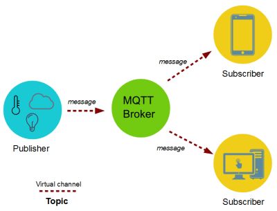
| Figure 2: Structure of MQTT |
If a broker receives a message on a topic for which there are no current subscribers, the broker discards the message unless the publisher of the message designated the message as a retained message. A retained message is a normal MQTT message with the retained flag set to true. The broker stores the last retained message and the corresponding QoS for the selected topic. Each client that subscribes to a topic pattern that matches the topic of the retained message receives the retained message immediately after they subscribe. The broker stores only one retained message per topic. This allows new subscribers to a topic to receive the most current value rather than waiting for the next update from a publisher.
When a publishing client first connects to the broker, it can set up a default message to be sent to subscribers if the broker detects that the publishing client has unexpectedly disconnected from the broker.
Clients only interact with a broker, but a system may contain several broker servers that exchange data based on their current subscribers' topics.
A minimal MQTT control message can be as little as two bytes of data. A control message can carry nearly 256 megabytes of data if needed. There are fourteen defined message types used to connect and disconnect a client from a broker, to publish data, to acknowledge receipt of data, and to supervise the connection between client and server.
MQTT relies on the TCP protocol for data transmission. A variant, MQTT-SN, is used over other transports such as UDP or Bluetooth.
MQTT sends connection credentials in plain text format and does not include any measures for security or authentication. This can be provided by using TLS to encrypt and protect the transferred information against interception, modification, or forgery.
The Things Network, commonly known as TTN, is an open-source infrastructure aiming at providing a free LoRaWAN network cover. This project is developed by a growing community across the world and is based on voluntary contributions to the project. Their website presents different guides to allow people to deploy gateways in their city to grow the network. These antennas provide both long-range coverage with LoRa and short-range with Bluetooth 4.2. Thanks to the open-source developments on the source code and on the infrastructure, their coverage is already quite good in big cities and it is spreading in smaller ones.
The Things Network uses MQTT to publish device activations and messages but also allows you to publish a message for a specific device in response.
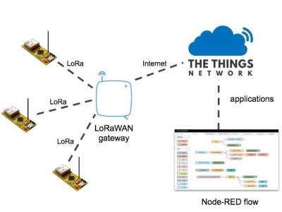
| Figure 3: Integration of the relevant technologies |
Node-RED is a programming tool for wiring together hardware devices, APIs and online services. It provides a browser-based editor that makes it easy to wire together flows using the wide range of nodes in the palette that can be deployed to its runtime in a single-click. The light-weight runtime is built on Node.js, taking full advantage of its event-driven, non-blocking model. This makes it ideal to run at the edge of the network on low-cost hardware such as the Raspberry Pi as well as in the cloud.
With over 225,000 modules in Node's package repository, it is easy to extend the range of palette nodes to add new capabilities.
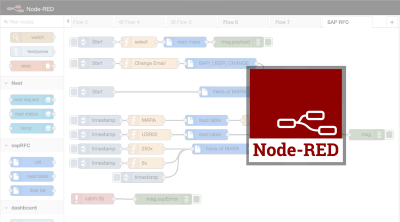
| Figure 4: Node-Red |
Node-RED consists of a Node.js based runtime that you point a web browser at to access the flow editor. Within the browser you create your application by dragging nodes from your palette into a workspace and start to wire them together. With a single click, the application is deployed back to the runtime where it is run.
The palette of nodes can be easily extended by installing new nodes created by the community and the flows you create can be easily shared as JSON files.
3. Concept
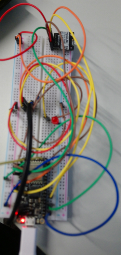
The entire technical stack that is used consists of different layers. On the one hand, we have the microcontroller and the Lora module and the antenna, which are used to forward measurement data. By means of Loawan, these data arrive as uplink messages in the ttn. There, the content of the uplink message is communicated to Node-Red using MQTT. Here, the forwarded uplink message becomes a “msg” that is usual for Node-Red. This is processed with the appropriate nodes and the extracted data is stored in the last step in Node-Red in Postgresql. The data serves as the basis for the visualization in Dash Plotly. Technically we use as microcontroller development board the adafruit feather M0 and two sensors to measure the temperature and distance. This also contains a lora module which works via SPI with the microcontroller and also a corresponding antenna for data transfer. Via IC2 the microcontroller gets the measurement data from the distance sensor VL53L1X.
| Figure 5: Hardware |
4. Implementation
4.1 Prototype and data transfer
4.1.1 TTN
After you have logged in to ttn, you have to click on the “Applications” section. Then you will be redirected and all registered devices will be listed. To register a new device, click on “Add Application”.
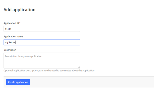
Then you can define an ID and name for the application and create the application. It should be noted that the ID must not be an ID that is already assigned and must contain only numbers, lowercase letters and dashes.
| Figure 7: Add application (details) |
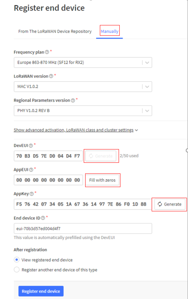
In the next step, a device can be assigned to the application by clicking “Add end Device”. The settings must be entered manually. Ttn automatically assigns an end device id. DevEUI and AppEUI have to be generated. The AppEUI is able to identify the owner of the end device. The DevEUI is used to identify the end device once. In the frequency plan the recommended frequency for Euroe should be chosen. The other parameters for the lorawan version and the regional parameter setting can be found in the datasheet of the used microcontroller.
| Figure 8: Register device |
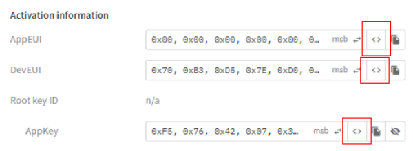
After the end device is created it can be clicked by user. Then a new page opens which contains all parameters for the end device. Here the data formats for the keys DevEui, AppEUI and AppKey can be formatted. It is important to note that the DevEUI and AppEUI keys are entered in the Little Endian Vormat in the script. AppKey is needed in the Big Endian Vormat. This works by pressing “Toggle array formatting” next to the keys. The symbol has been outlined in red in the next figure.
| Figure 9: Change data format |
4.1.2 relevant libraries and sketches
The following libraries should be installed under Tools → Manage Libraries:
- MCCI LoRaWan LMIC library
- SparkFun VL53L1X 4m Laser Distance Sensor
- DallasTemperature
“MCCI LoRaWan LMIC library” is used for the transmission of the measurements to the ttn. “SparkFun VL53L1X 4m Laser Distance Sensor” is used for the programming of the distance sensor and “DallasTemperature” is used for the programming of the temperature sensor.
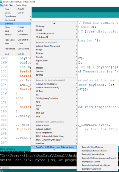
The final sketch that was used is just a mix of different example sketches. The following example sketches were used as a inspiration for the final sketch:
- ttn-otaa (MCCI LoRaWan LMIC library)
- Example1_ReadDistance (SparkFun VL53L1X 4m Laser Distance Sensor)
- simple (DallasTemperature)
How to open an example is illustrated in the next figure.
| Figure 10: How to open the examples |
4.1.3 Embedded programming
At the beginning of the script the previously defined keys must be specified, because without these keys no authentication is possible. OTAA was explained in detail at the beginning of the documentation, so parts of the code that deal with activation are only briefly mentioned.
| Figure 11: Implementation of the keys |
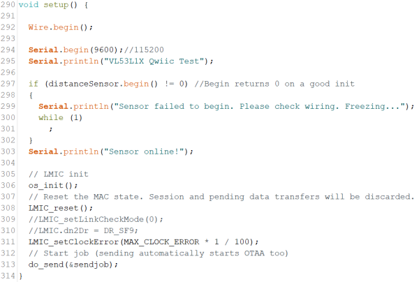
Most of the important things happen in the do_send, onEvent and setup functions. “setup” is used to test wheather the distance sensor is available and initialize LMIC.
| Figure 12: setup function |
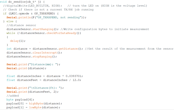
The do_send function is the most relevant function because the data for transmission in ttn are prepared there. All measured values are received there and prepared as bytes for sending. If no transmission is currently running, distance data is retrieved and stored as byte.
| Figure 13: get distance and store as byte |
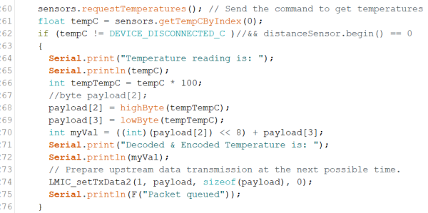
The same principal is applied to the temperature data. Here you have to take care that the temperature is integer, therefore the temperature is multiplied by 100.
| Figure 14: get temperature and store as byte |
“onEvent” reacts on different events that can occur. For example it is used to handle events that are relevant for the authentication and activation of the device.
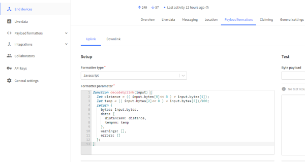
After the data has entered the ttn via an uplink message, the high and low bytes must be decoded so that both the high byte and the low byte are in the correct position. Furthermore the temperature has to be calculated again to a decimal number by dividing by 100.
| Figure 15: Decoding |
The incoming data is then displayed in the “Live data” section.
| Figure 16: Select live data |
The pin configuration to ensure a successful SPI communication between the microcontroller and the Lora module must be done exactly as shown in the next picture.
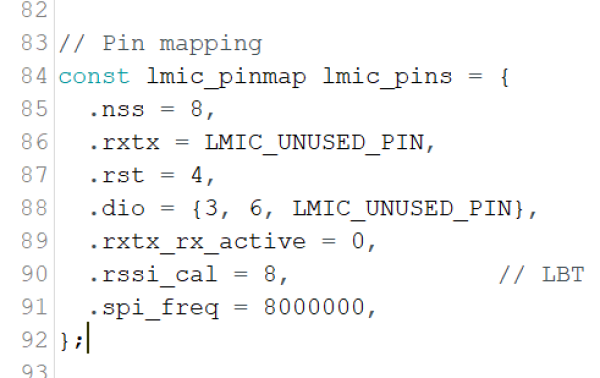
| Figure 17: Pin configuration |
4.2 Implementation in Node-Red
4.2.1 "Theoretical" test with 3 gateways
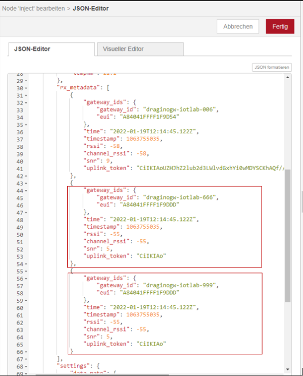
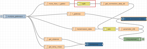
The entire flow starts with an injection node which contains a payload consisting of a file which was created by TTN. The only difference is that for testing purposes several gateways were added to the file.
The first gateway is the gateway from the original message, all other gateways and their ids were made up to test the entire flow and database. The initial injection node containing the modified json file has five connections to other nodes.
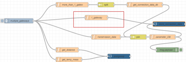
| Figure 19: Flow for “one” gateway |
The simplest case is that a message is only received from one gateway. In this case the function “1_gateway” contains all gateway and connection data.
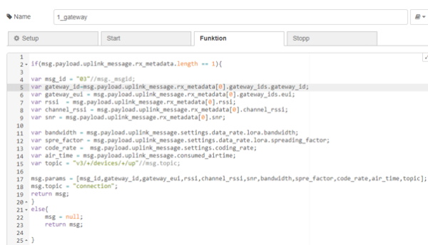
| Figure 20: Function 1_gateway |
These parameters are extracted individually from the payload and assigned to new variables. This happens only if the array “msg.payload.uplink.rx_metadata” has the length one, i.e. contains only one gateway. If more gateways are contained, msg is initialized with null and nothing is stored in the database. The newly set variables are stored in “msg.params”. “msg.params” contains the parameters which will be used in the following postgresql-node.
| Figure 21: Store connection data |
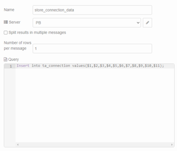
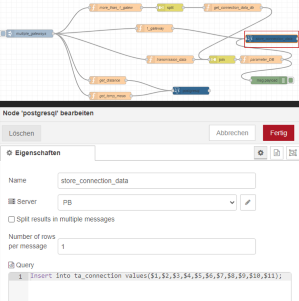
The set parameters are the input for the insert statement within the node.
| Figure 22: Insert statement with the necessary parameters |
This saves the previously defined values in the database in the table “ta_connection”. For the postgreql node some settings must be made so that the database can be used.
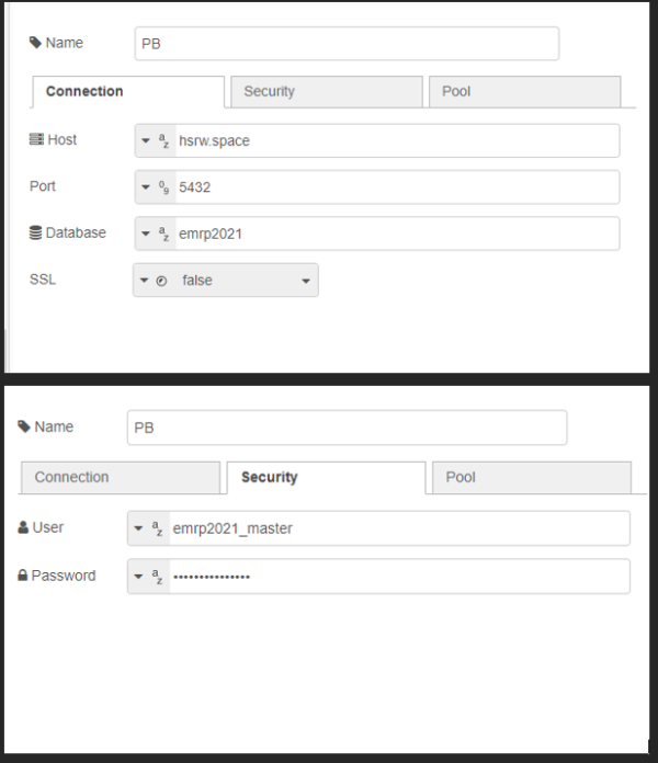
| Figure 23: Settings for the database |
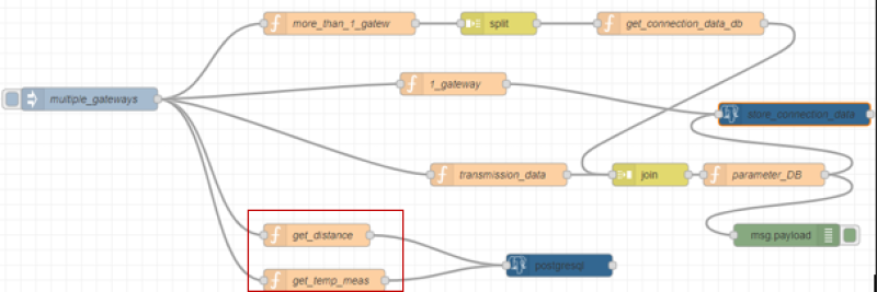
Firstly, the host and the database used must be specified. Also, the database user and the password of the database must be specified. However, it should be noted that if one postgresql node is changed then all postgresql nodes are automatically changed. The measured values for the distance and the temperature are extracted by the nodes “get_distance” and “get_temp_meas” from the payload of the initial json file.
| Figure 24: Functions to extract data for the measurement tables |
Both functions are designed to extract data only if measured values are available, otherwise msg is set to zero.
| Figure 25: Details for get_distance |
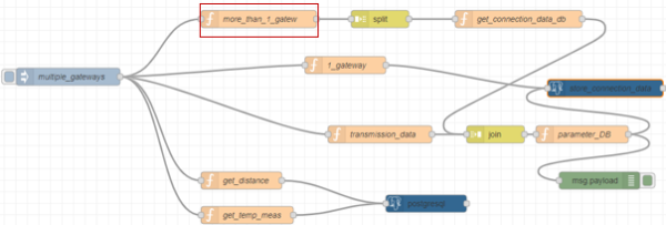
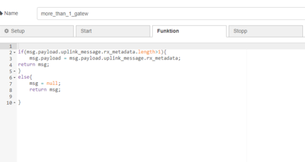
Similar to the example before, the necessary parts of the payload are extracted here and set as parameters for the following query. This was illustrated for “get_distance” in the figure but the same principle can be found in “get_temp_meas”. However, transferred json files that have multiple gateways are a bit more complicated. The function “more_than_1_gatew” checks if the object contains more than one gateway and initializes the payload with the object for the gateways. If not, msg is initialized with null.
| Figure 26: Function node to handle more than one gateway |
| Figure 27: Details for “more_than_1_gatew” |
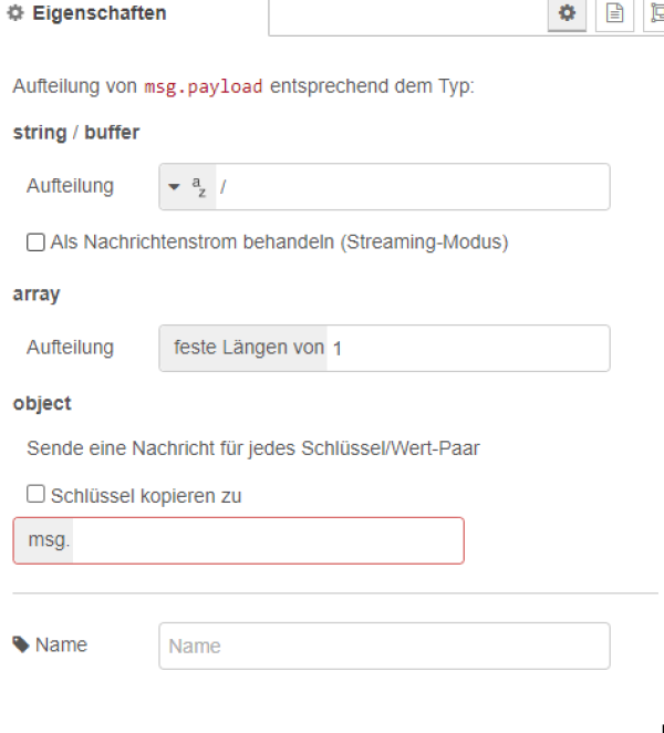
The node “split” ensures that the payload is always split off as an array with the length one, so that, for example, an object containing 3 gateways is split three times into three payloads.
| Figure 28:split node |
| Figure 29: Details for the split node |
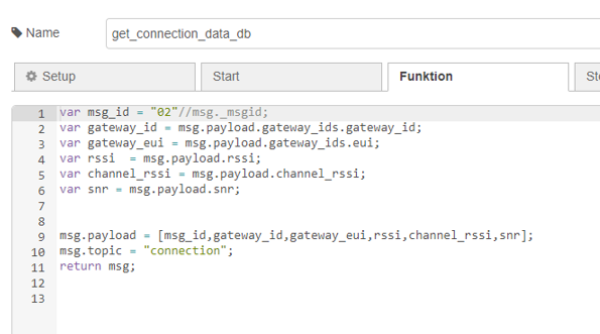
After that each payload is forwarded in the flow to the function “get_connection_data_db”. There the relevant parts of the split objects are extracted and stored in the payload as an array. It is important that “msg.topic” is also provided with a unique value. This will be important for the next join node.
| Figure 30: Details for the function “get_connection_data” |
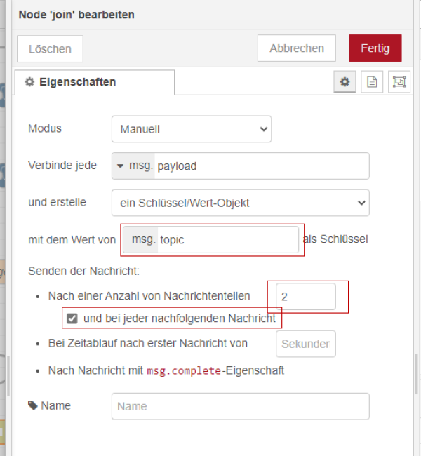
In the join node, the gateways are combined with the connection data. This results in data sets with the same connection data but different gateway information. With the use of the join Node is to be considered that the individual message parts must set in each case unique msg.topics before and that with the properties of the join Node the number of the message parts is specified and also the hook “and with each following message” is set. If this is not done the join node may not be able to process more than 2 separate gateway information. All joined data will be stored as a value object.
| Figure 31: Properties of the join node |
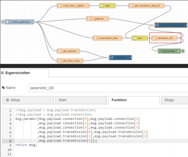
Then the function “parameter_DB” is used to extract all values from the merged object. For this the msg.topics “connection” and “transmission” defined before are used.
| Figure 32: Parameters based on the topics connection and transmission |
At the end, the defined parameters from msg.params are inserted into the insert-statement. It is important to note that the number of times the query is executed after the initial injection depends on how many gateways were split from the initial object. For example, if three gateways were split from the object then the query will also be filled three times with different parameters for the gateways.
| Figure 33: Insert statement |
4.2.2 real prototype
The real prototype is quite similar to the test example. But it is not using an injection node anymore.
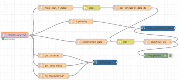
| Figure 34: Prototyp |
Instead a “mqtt in” node is used which receives the data from ttn.
| Figure 35: MQTT in node |
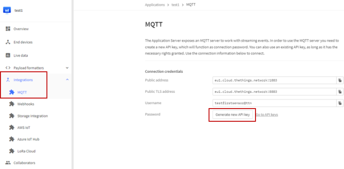
To send a message via MQTT from ttn to Node-Red, the MQTT server of ttn must be used. For this, an API key must be created in ttn. MQTT configuration can be accessed via “Integrations”.
| Figure 36: How to generate API key for MQTT |
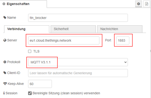
After that “Generate new API key” can be clicked to generate a new key. This allows to use the MQTT server. From the last figure, the server and the port can also be copied from the field “Public address” and can be put within the properties of the MQTT Node. Also the used protocol must be specified within the properties in our case it is “MQTT V3.1.1”.
| Figure 37: connection parameters |
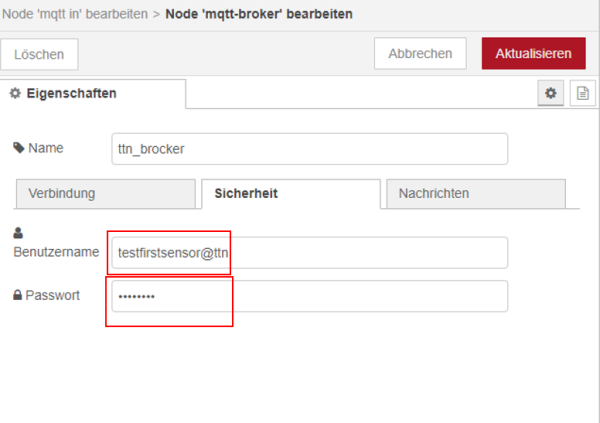
Furthermore, both the generated API key as password and additionally the username have to be provided. Both can be seen for example in figure 35 for this project and have to be added to the properties of MQTT node.
| Figure 38: integration of password and username |
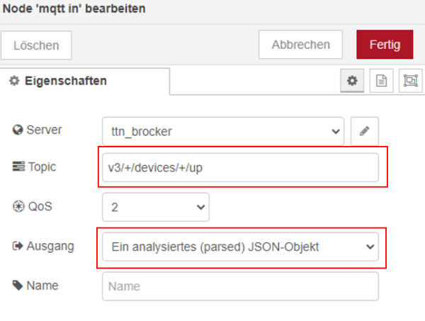
The only part that is missing is the implementation of the topic to retrieve messages from the uplink traffic. The topic used is a topic provided by the MQTT server. Wildcards are used for the application_id and the device_id. This allows Node Red to receive messages not only from one device. Furthermore, json object must be selected as output.
| Figure 39: Set output and right output |
4.3 Datamodel
4.3.1 Tables
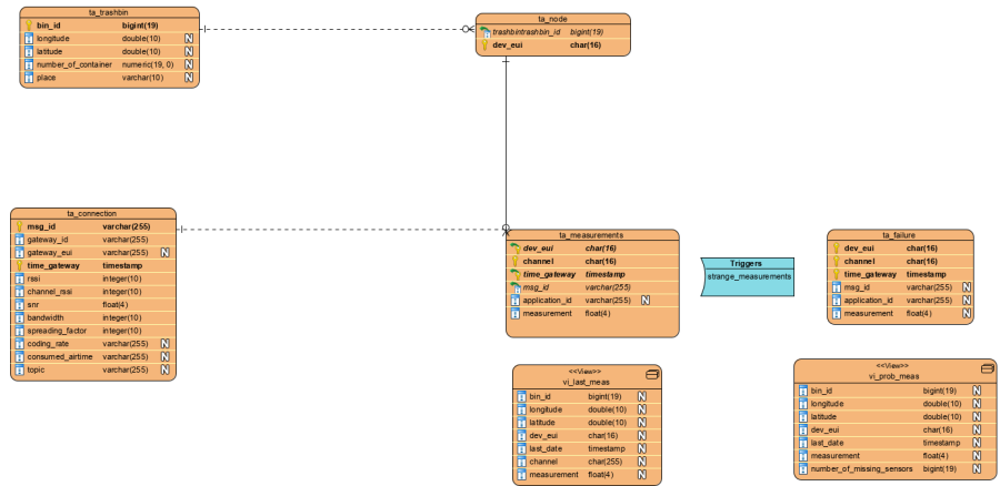
The database we use consists of static and dynamic tables.
| Figure 40: Used tables and views |
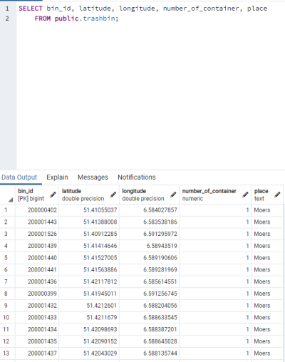
Among the static tables, we have, among others, the table “ta_trashbin”, which stores all trash bins, their location, number of containers, and the city in which they are located. “bin_id” acts as the primary key for this table.
| Figure 41: Table for the trashbins |
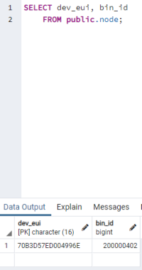
The other static table is “ta_node”. This stores all active devices and their associated trash bins. “dev_eui” is the primary key and “bin_id” is the foreign key of the table. The table must be updated every time when a new device is attached to a trash bin. Otherwise, no new measured values can be stored.
| Figure 42: Table for the node |
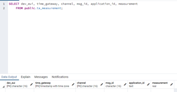
To the dynamic tables, which are filled by new measured values, belongs “ta_measurement”. This contains only the measured values for the respective sensors. The primary key consists of the columns “dev_eui”, “time_gateway” and “channel”. Channel indicates which measurement type is present.
| Figure 43: Table “ta_measurement” |
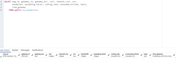
The next dynamic table is “ta_connection”. This uses the “msg_id” and “time_gateway” as primary keys. The table consists of columns that refer to the respective gateway (gateway_id, gateway_eui, rssi, channel_rssi, snr, time_gateway) and the other columns refer to the transmission of the data.
| Figure 44: Table “ta_connection” |
4.3.2 Views and Trigger
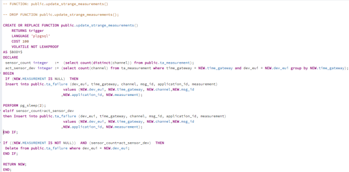
“ta_failure” is a table that is structured in the same way as “ta_measurement”. It is also indirectly filled by “ta_measurement” by using an insert trigger. This stores questionable new records also into the “ta_failure” table.
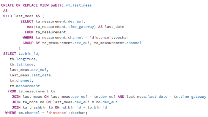
Beside the tables there are also two views which serve as bases for Dash Plotly. “vi_last_meas” has the last measurement for each microcontroller.
| Figure 45: View “vi_last_meas” |
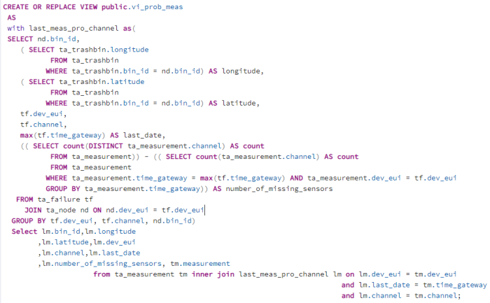
“vi_prob_meas” has the latest problematic record for the microcontrollers. In case of missing sensor measurements, the number of missing measurements is displayed in the last column.
| Figure 46: View “vi_prob_meas” |
The trigger checks two things firstly whether the data records contain measured values, if not the data record is also written to the failure table. The next condition that is checked is whether all sensors were taken into account during the transmission of the data records. If not, the data records are written into the failure table. If new data records appear that are free of errors, the old data records are deleted from the failure table.
| Figure 47: Insert-Trigger after each insert |
4.4 Dash Plotly
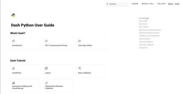
Plotly develops Dash and also offers a platform for writing and deploying Dash apps in an enterprise environment.
| Figure 48: Dash User Guide |
What is Dash?
- Dash is a Python framework for building web applications.
- Dash is simple enough that you can bind a user interface to your code in less than 10 minutes.
- Dash is the original low-code framework for rapidly building data apps in Python, R, Julia, and F# (experimental).
Why Dash?
- Dash is ideal for building and deploying data apps with customized user interfaces.
- It enables you to build dashboards using pure Python.
- Dash is open-source, and its apps run on the web browser.
Dash Installation
In order to start using Dash, we have to install several packages.
- The core dash backend.
- Dash front-end
- Dash HTML components
- Dash core components
- Plotly
Dash App Layout
A Dash application is usually composed of two parts. The first part is the layout and describes what the app will look like and the second part describes the interactivity of the application. Dash provides HTML classes that enable us to generate HTML content with Python. To use these classes, we need to import dash_core_components and dash_html_components. You can also create your own custom components using Javascript and React Js.
In order to get started, we will create an app.py file in our favorite text editor, then import the packages mentioned.
| Figure 49: Import Libraries |
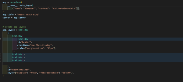
When we initialize Dash, we call the Dash class of dash. After that is done, we create an HTML div using the Div class from dash_html_components. Dash_html_component has all HTML tags, and dash_core_components has Graph, which renders interactive data visualizations by using plotly.js. The graph is used to create graphs on our layout. Dash also allows you to style the graph by changing colors for the background and text. Graph classes expect a figure object with the data to be plotted and the layout details. If you use the style attribute and pass an object with a specific color, you can change the background and so on.
In the figure below you will see how our layout is structured and what's included.
| Figure 50: Dash Layout |
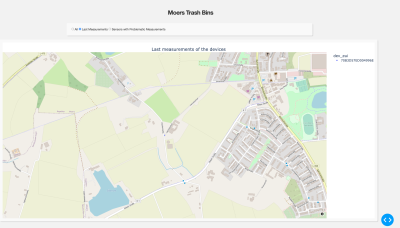
Dash apps use callback functions to update the properties of another component when an input property changes. In-Dash, any “output” can have multiple “input” components. And in our example, we are going to use multiple-input call back functions for example we had one callback function that take two inputs (intervals and data_type) and display one output as a graph output of what we have done for the trash bins measurements in Moers as you will see below in the below following figures.
| Figure 51: All Trash Bins Located in Moers |
in the above figure, you will be able to see all implemented trashbin with all information about them as ( location of trashbin, trashbin id)
As can be seen in the below image, we display only the latest measurements from the active sensors upon request of the user, which we use as an input to a call-back function.
| Figure 52: Last Measurements |
In the below figure you will show more detailed information about our project
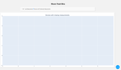
| Figure 53: Problemetic Measurements |
Finally, remember that Dash is built on top of Flask, so the webserver needs to be running just like Flask for us to view our visualization. We also set debug to true so no fresh server is needed every time we modify the visualization.
| Figure 54: Main Function |
For our project, this is not enough for that reason we do some extra programming stuff that allows us to grab data from the database and display it. So for that, we prepared the following queries script file which facilitates our working and allows us to be connected to our own database which is built-in progress as seen below
| Figure 55: Database Connection |
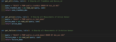
then we define some functions which allow us to get needed information from the database as you will see in the figures below
| Figure 56: Queries Part 1 |
| Figure 57: Queries Part 2 |
And now we can say that everything is done regarding the dash plotly part in our project.
5. Dynamic pivot and Dash Plotly
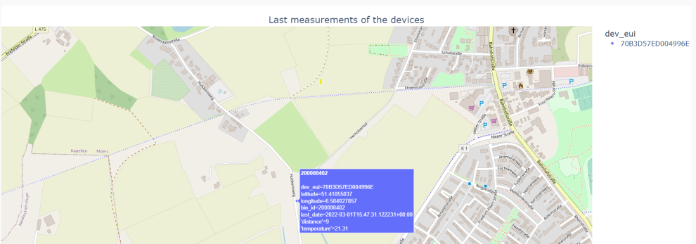
In the representation of the second map presented so far, which contains the last measurements for each device, only the last filling levels are taken into account. All other measured values are not considered. In order to be able to display all measured values and also new values based on new sensors, two basic requirements must be met. First, the measured values must be aggregated and then pivotoized. In the second point, it must be ensured that if a measurement type is added, this is also dynamically taken into account in the pivoted representation.
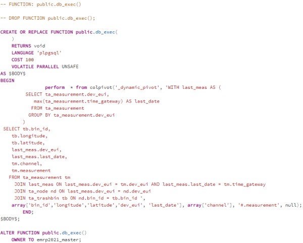
After an intensive research we have found a prescribed function which is able to fulfill our requirements with few restrictions. The original function which can also be found under the link in the last section creates temporary tables which are deleted after execution. In our approach we have changed this point. A table is created and based on this table a view was created.6 parameters are passed. The first parameter is the name of the new view. The second parameter is the query used for the table of the view. The third parameter contains columns that represent the reference columns that will be used for pivoting. New columns are specified by using the fourth parameter. The last two parameters define the content which can be found in the new columns and it is also possible to define a order for all columns. The only disadvantage is that the table used for the pivotized view has to be deleted every time the function is called, the same is true for the view.
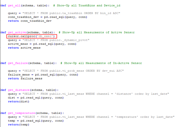
Dash Plotly had to be adapted as well. Every time the map is updated for the latest readings, the function must also be called to create a new table and view. In our case it is the function 'db_exec'.
| Figure 58: Funtion db_exec |
The function has no parameters but serves to call the original function 'colpivot' with the parameters. The nesting of the functions was done because the specification of the parameters in Python is very complex.
| Figure 59: Call of the function db_exec |
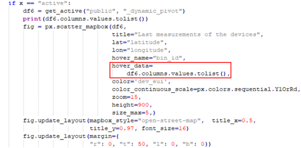
As a result, it is now possible to call up the last measured values for each device in a pivoted manner, instead of having to decide on a measurement type as in the previous version, it is now possible to call up the last date and the corresponding measurements for all devices.
| Figure 60: last measurement per device |
In order for it to work, all columns must always be displayed, instead of defining only some columns statically, as was done in the previous version.
| Figure 61: choose all columns |
6. Links and Tutorials
- CODE used in the project: https://github.com/ubaidadib/EMRP_WS_2021_Project
- Mix-Playlist about different topics: https://www.youtube.com/playlist?list=PL2SRmCaIeDVibo6IUItyKcmDCH955hqAT
- Link for ttn: https://www.thethingsnetwork.org/
- SQL-Querries (Postgresql) in Node-Red: https://flows.nodered.org/node/node-red-contrib-postgresql/in/MFnap-qr-MJE
- TTN, MQTT Node-REd: https://www.thethingsindustries.com/docs/integrations/mqtt/
- dynamic pivoting using Postgresql PL/PGSQL: https://github.com/hnsl/colpivot

